Wide Field Infrared Camera for UKIRT

UKIRT WFCAM - Optical Design

Conceptual Design Review, August 1999

David Henry

1. Introduction

This document describes the optical design for the proposed Wide Field Camera (WFCAM) for the UK Infrared Telescope (UKIRT). It is presented as part of the conceptual design review for the instrument.

2. Specification

The optical system specifications for the WFCAM are taken from the top level requirements document. Here we summarise the baseline optical specifications.

• Broad band imaging in J,H and K bands
• Field of view of 0.93° diameter
• Pixel scale of 0.4 arcsec/pixel (18µm pixels)
• Image quality of better than 0.26 arcsecond RMS blur diameter
• Cold stop for K-band imaging

The following wavebands are assumed for J,H and K.

3. Optical Layout & Description

Figure 1 below shows an optical layout of the WFCAM optical system. Figure 2 shows a close up of the cryostat optics.

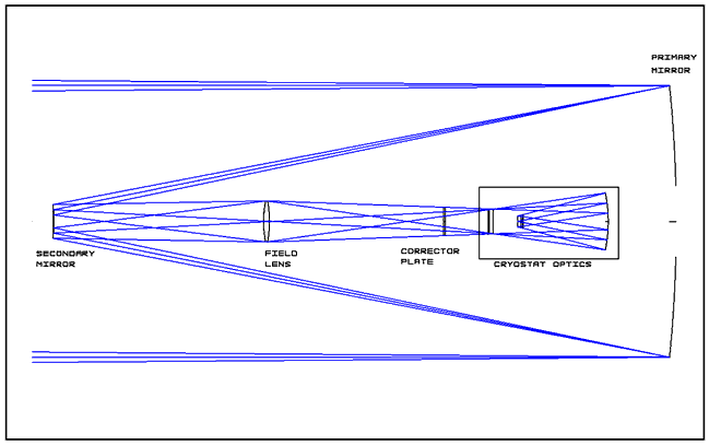
Figure 1 - WFCAM Optical Layout

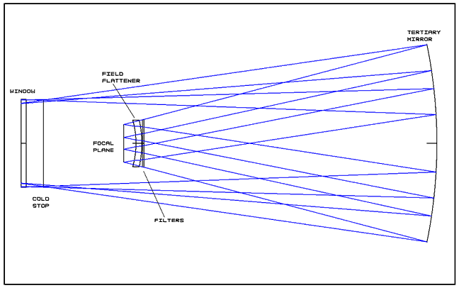
Figure 2 - WFCAM Cryostat optical layout

WFCAM uses the existing UKIRT primary mirror (paraboloid, 3.8m diameter, F-ratio f/2.5). The primary mirror forms the aperture stop for WFCAM.

A new secondary mirror produces an f/9 focus, at a distance of 5.767 metres in front of the primary mirror. The secondary mirror is hyperbolic (radius of curvature -2231mm, conic constant -3.308) and is approximately 472mm in diameter (approximately 50% larger than the current UKIRT secondary).

At the intermediate focus, a fused silica field lens is placed. This is used to re-image the primary mirror onto a convenient cold stop. The field lens is bi-convex (spherical surfaces), and is approximately 580mm in diameter, by 80mm thick

The next optical element is an aspheric corrector plate. This is made from fused silica, 400mm in diameter by 20mm thick. One side of the plate is flat, and the other side has a weak aspheric profile, similar to a Schmidt plate. This plate corrects residual aberrations in the system.

The cryostat window is next. This is a plane parallel fused silica window, of diameter 180mm. The exact thickness of this window will be determined via an analysis of the likely vacuum loading, and the need to minimise the resulting deformation of the surface. This will be the subject of a fuller analysis in the next phase of the project. The window thickness is likely to be a minimum of 20mm.

Just inside the cryostat, an image of the primary mirror is produced. The cold stop is located here.

The tertiary mirror is located at the rear of the cryostat. This converts the f/9 beam from the secondary mirror into the f/2.44 beam required to give the correct pixel scale. The tertiary mirror is a concave hyperboloid (radius of curvature -1993mm, conic constant -0.0819) of diameter 800mm.

The beam then passes through the filters - these are discussed in more detail in section 6.

Directly in front of the focal plane is a fused silica field flattening lens. The lens is a meniscus, with spherical surfaces. This lens reduces the field curvature of the system.

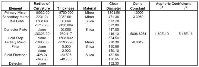
Appendix 1 contains a complete optical prescription for the WFCAM baseline design.

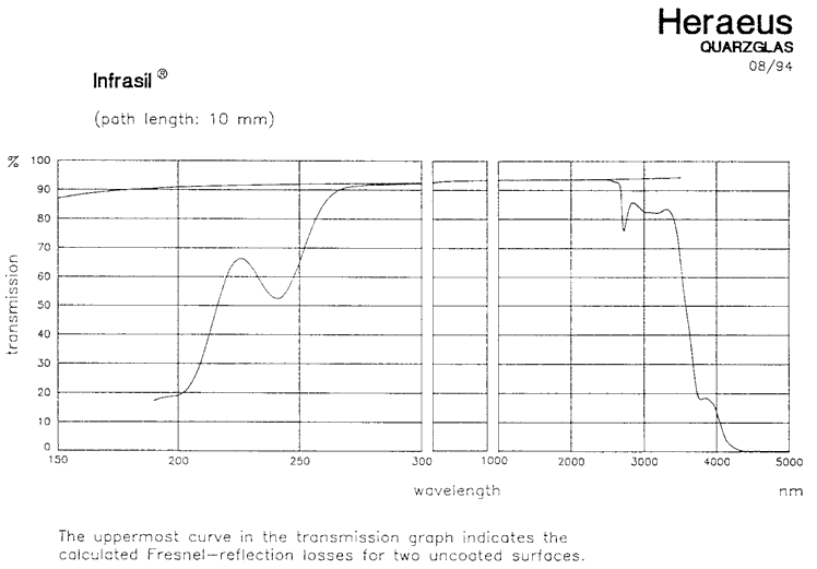
4. Optical Materials

All of the refractive elements in the system (field lens, corrector plate, window and field flattener) are made from fused silica. This is available in various types and grades. For example, Infrasil 302 from Heraeus provides material with good refractive index homogeneity, extremely low counts of bubbles and inclusions and transmission out to 2.5 µm. Fused silica is readily available in large blank sizes, suitable for fabrication into the lenses required for WFCAM.

The graph below shows the transmission of Infrasil 302.

The secondary mirror will probably be fabricated from Zerodur, similar to the existing UKIRT secondary mirror. This represents the low risk approach, since the current secondary mirror is known to perform well.

There are a number of choices for the substrate material for the tertiary mirror, the main choices being aluminium alloy, Zerodur and Silicon Carbide. The final choice of material for this element will be decided by a trade-off study in the next phase of the project. This study will examine all aspects of the tertiary mirror (including cost) to arrive at the optimum choice for the material.

5. Throughput, transmission and vignetting

Figure 3 below shows the vignetting (caused by the hole in the primary mirror and the obscuration of the focal plane) as a function of field angle. The plot is for J band - H and K band plot are similar.

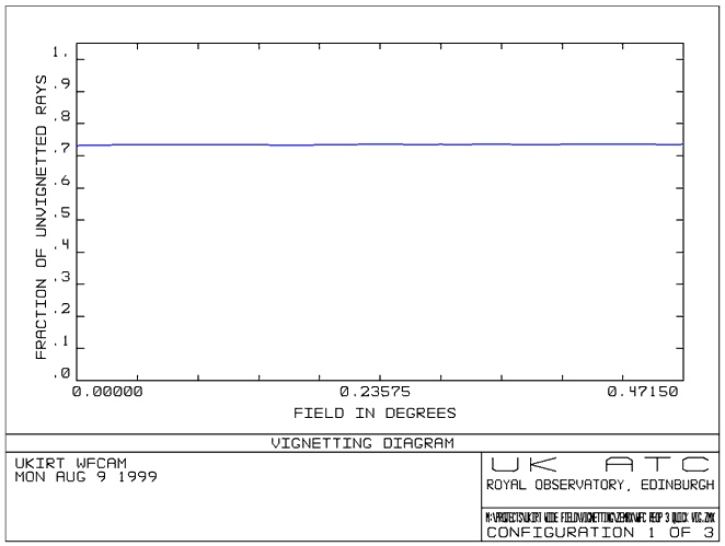
Figure 3 - Vignetting plot

The vignetting in the system is estimated at around 27%, with little variation across the field of view.

Tables 1 and 2 below show maximum and minimum estimates of the transmission through the system.

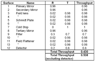Table 1 - Maximum transmission estimate	Table 2 - Minimum transmission estimate

The maximum transmission estimate is based on 98% reflectivity for mirrors, 1% reflectivity for lenses and 80% transmission for the filters. Minimum transmission assumes 96% mirror reflectivity, 2% lens surface reflectivity and 70% filter transmission. The detector is assumed to have a 20% reflectivity - this is included as these tables are used in the analysis of ghost imaging - see section 8.

Using these figures we get an estimate of transmission of between 53.8% and 70.2% (excluding the detector. Combining this with the 73% from the vignetting analysis gives an overall throughput of between 39.2% and 51.2%.

6. Filters

The IR filters are mounted directly in front of the field flattening lens. This minimises the size of the filters, thereby minimising the obscuration of the beam. Figure 4 below shows an optical layout of the filters. Figure 5 shows a beam footprint on the front surface of the filter. Beams are shown from the four corners of three of the four individual detector arrays (a limitation in ZEMAX restricts the number of field points to 12, meaning that only beams from three of the four detectors can be shown).

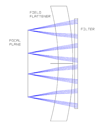
Figure 4 - Filter Optical Layout

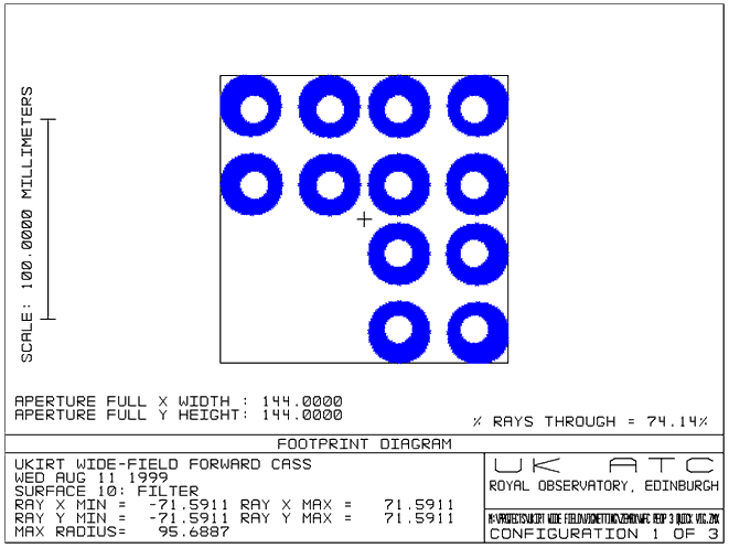
Figure 5 - Beam footprint on filter surface

From the footprint diagram we can see that the footprints from each individual detector do not overlap at the filter surface. We can therefore use four separate filters mounted in a structure to form a 2x2 pattern. This significantly reduces the manufacturing risk and cost associated with the filters.

For the baseline preliminary design, each individual filter is approximately 75mm square. The filters will be fabricated from fused silica, of a similar grade to that used for the lens elements.

7. Optical Performance

The plots below show spot diagrams for the WFCAM system, in J, H and K bands.

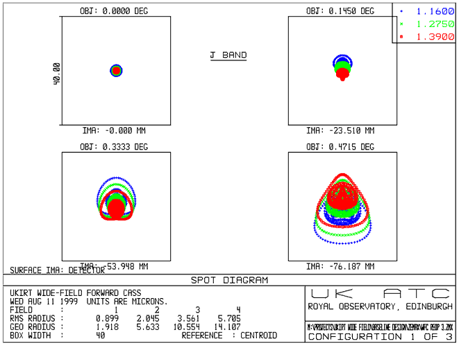
Figure 6 - Spot Diagram (J Band)

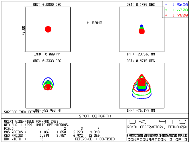
Figure 7 - Spot Diagram (H band)

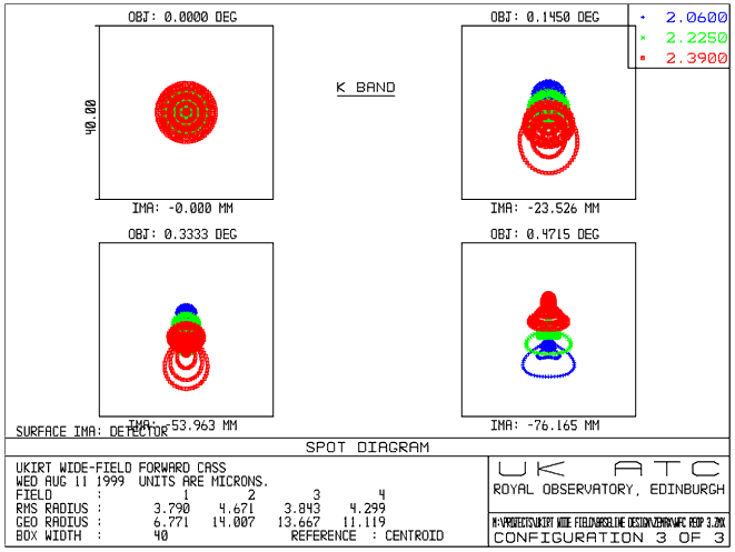
Figure 8 - Spot Diagram (K Band)

The field points are chosen to represent the inner corner, the edge and the outer corner of the four detectors (see diagram below). Note that the 0° field position is not actually imaged by the detector arrays.

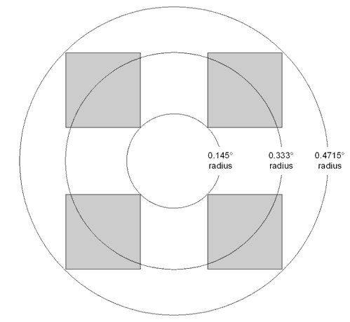
Figure 9 - Focal plane and field of view

The graph below shows the variation of RMS optical blur diameter (in arcsec) with field angle for each of J, H and K bands. As can be seen from the graph, the nominal performance of the system exceeds the specification at all field angles and wavebands.

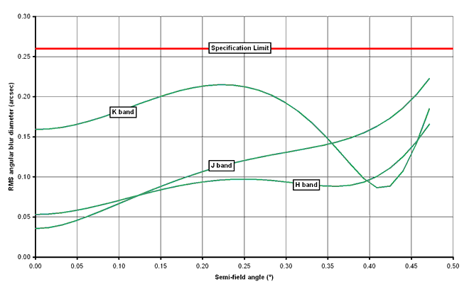
Figure 10 - RMS blur diameter vs. field angle

Note that this calculation of RMS spot size does not include any diffraction effects. To get an idea of the effects of diffraction, we can look at the encircled energy.

The plots below show the diffraction encircled energy up to a radius of 18mm for J,H and K wavebands. The calculations are performed on axis, at 0.33° (edge of field) and at 0.4715° (corner of field). These calculations include the effects of diffraction from the central hole of the primary mirror and diffraction from the focal plane.

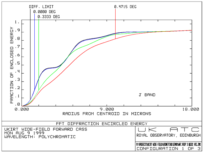
Figure 11 - Encircled Energy (J Band)

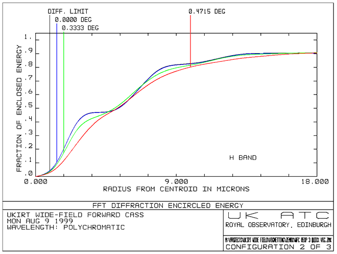
Figure 12 - Encircled Energy (H Band)

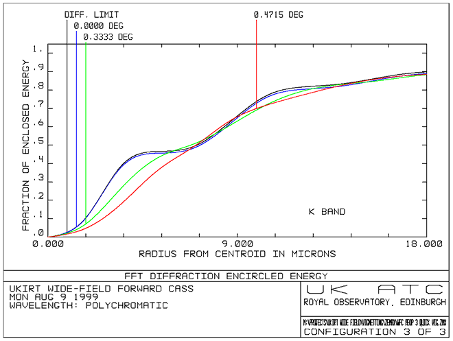
Figure 13 - Encircled Energy (K band)

We can see that the effects of diffraction are most noticeable at K band.

The plot below shows the percentage image distortion as a function of field angle for three wavelengths (which are roughly the central wavelengths for J, H and K).

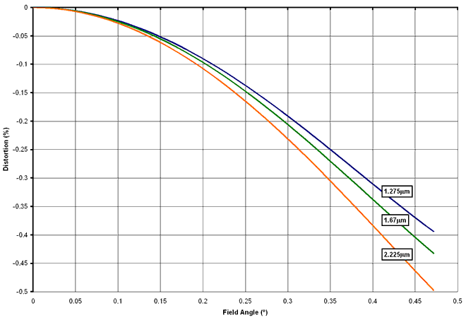
Figure 14 - Image Distortion

The worst case distortion is 0.5% at the corner of the field of view in K band. This corresponds to an image shift of 0.762mm, or 42 pixels. Image distortion will require correction in software when individual frames are "stitched" together to form an image.

8. Ghost Imaging

An initial ghost imaging analysis has been performed. The analysis looked at on axis ghosting only, and considered double bounces in the system (i.e. light coming in from the sky is partially reflected from a surface, back towards another surface, then reflected again towards the focal plane).

The procedure adopted is as follows.

- A ray tracing analysis is used to calculate the radius of each of the ghost images on the focal plane (rghost).

- The area of the ghost image is then calculated (Aghost).

- The overall transmission through the complete optical path forming each ghost is then calculated (Tghost). This takes account of all multiple reflections, and includes detector reflectivity at 20%. The values used are those shown in Table 1 - Maximum Transmission Estimate in section 5.

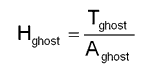
- The nominal irradiance in the ghost image (for an nominal incident power of 1W in the aperture, and assuming that the power is spread evenly across the defocussed ghost image) is then calculated as:

- For comparison, the diffraction limited irradiance on the focal plane for a point source illuminating the aperture with a power of 1W is calculated (this is just the peak intensity for the Airy disk function for a circular aperture). This is calculated as:

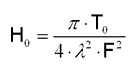
where:

= nominal transmission through system (including detector reflectivity) = 0.561

= wavelength = 1.5mm

F = optical f-number = 2.44

(Reference - V.N. Mahajan, "Aberration theory made simple")

- The relative irradiance of each ghost image is then calculated as

The table below shows the ghost radius and area, throughput and relative irradiance for ghost images produced by the surfaces in the system.

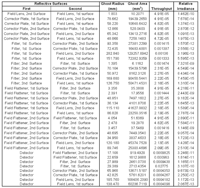
Table 3 - Ghost Image Analysis

A number of conclusions can be drawn from this analysis.

• The highest intensity ghost images are those produced by reflections from the filters, which have the highest surface reflectivity. However, these are of the order of 109 lower in intensity than the primary image.
• The smallest radius of ghost image is >1mm in diameter.
• The analysis above was done using a previous design which did not incorporate a window. Ghost images from the window are expected to be of the same size and intensity as those produced by the corrector plate.
• The raytracing analysis does not correctly handle "second bounces" from the reflective surfaces in the system (primary mirror, secondary mirror and tertiary mirror). However, a manual analysis shows that ghost images produced by these surfaces are highly defocussed. Therefore, these are not included in the analysis shown above.

In conclusion, this first order analysis shows that the system should not be susceptible to ghost imaging, at least to first order. This is mainly a consequence of the fast F-ratio of the system, which translates into a correspondingly small depth of focus. This means that ghost images rapidly defocus (and lose intensity) as the focal point moves away from the focal plane.

In the next phase of the project, a fuller analysis of all aspects of stray light, including off-axis ghosting will be carried out.

9. Tolerancing

An initial tolerance sensitivity analysis has been carried out on the system.

9.1 Results of Sensitivity Analysis

Table 4 below shows which parameters are considered in this analysis, and how the effect in performance is judged.

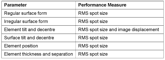
Table 4 - Tolerance Sensitivity Parameters

Notes:

• RMS spot size is calculated as the RMS spot radius in microns, on the focal plane. Only geometrical aberration effects are included.
• RMS spot size is measured on axis and at a field angle of 0.333° (the edge of the field).
• Highlighted cells in the sensitivity tables show changes of >0.5% from the nominal value.
• This analysis was performed with an early version of the design, which did not include the window.
• No analysis has been performed at this stage of the various aspheric coefficients of the secondary mirror, the corrector plate and the tertiary mirror.

9.1.1 Regular Surface Form Error

The table below shows the effect of a change in the regular surface form on the RMS spot size. These correspond to a change in radius for a spherical surface, or a sphericity on a nominally flat surface.

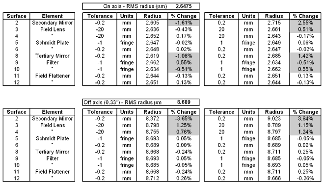
Table 5 - Sensitivity to Regular Surface Form Error

We can see from the table that the most sensitive elements are the secondary mirror and the tertiary mirror. These will require particular attention during the detailed tolerancing analysis. The field lens is particularly insensitive (since it is close to a focus) - this is fortunate since the field lens is large, and therefore difficult to manufacture.

9.1.2 Irregular Surface Form Error

The table below shows the effect of a change in the irregular surface form error on the RMS spot size. This can be thought of as departure from sphericity for a nominally spherical surface (e.g. astigmatism).

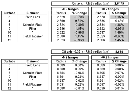
Table 6 - Sensitivity to irregular surface form error

None of the sensitivities for irregular form look particularly worrying at this stage. The difficulty is likely to arise in maintaining these tolerances over the large diameters of some of the optics.

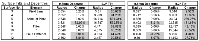
9.1.3 Element tilt and decentre (image quality)

The table below shows the change in RMS spot size with element tilt and decentre. These sensitivities correspond to the mechanical mounting and alignment tolerances.

The "cryostat optics" comprise the corrector plate, the tertiary mirror, the field flattener and the focal plane. These are grouped together and acted on as a single element.

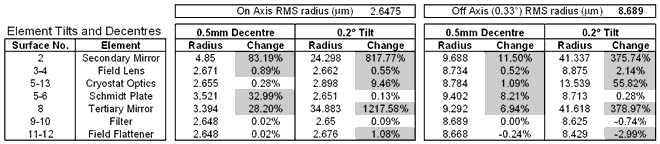
Table 7 - Sensitivity to element tilts and decentres

We can see that some of the elements listed are extremely sensitive to tilt and decentre, which will mean correspondingly tight manufacturing and alignment tolerances. In particular, the secondary and tertiary mirrors are sensitive to tilt misalignment.

9.1.4 Element tilt and decentre (image displacement)

The table below shows the image displacement on the focal plane for small changes in element tilt and decentre.

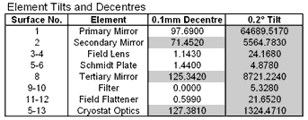
These sensitivities are useful in determining the likely image motion due to mechanical flexure of the instrument.

9.1.5 Surface tilts and decentres (image quality)

The table below shows the change in RMS spot size with surface tilt and decentre. This corresponds to the wedge angle of a lens, for instance.

The largest sensitivities are on the tilt of the corrector plate (Schmidt Plate) surfaces. However, the wedge angle used for the sensitivity analysis (0.2°) is large when compared to normal optical fabrication tolerances.

9.1.6 Thickness and Separation

The tables below show the change in RMS spot size when element thicknesses and element to element spacings are varied. The analysis is performed with and without back focus compensation. In addition, in certain cases, thickness compensation is used. This accounts for the fact that when a lens element is increased in thickness, it will "expand into" the next air space.

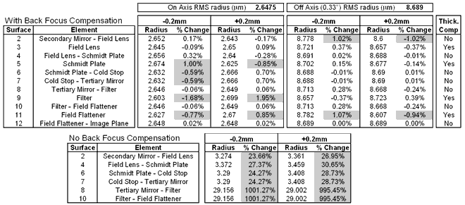
As would be expected, when the system is not re-focussed, the degradations in image quality are larger. Using back focus compensation in this analysis is not strictly correct, since there will be no focus mechanism. However, using back focus compensation gives us an idea of the amount of one-off adjustment that will be necessary.

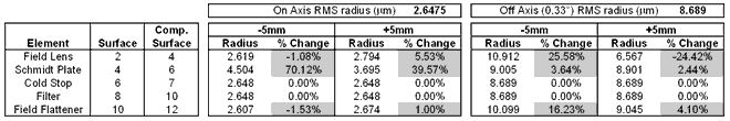
9.1.7 Element Position

The table below shows the change in RMS spot size when the optical elements are moved by small amounts along the optical axis. (NB. This differs from the previous analysis which looked at changes in separation of two elements. Here, compensator surfaces are used to model the effects of changes in position).

9.2 Key Conclusions from Sensitivity Analysis

The following conclusions can be drawn from this analysis.

• Some of the alignment tolerances with regard to tilt and decentre of optical components are highly sensitive. In particular, the alignment of the primary, secondary and tertiary mirrors is critical. Due to the large field of view of the system, any image degradation due to a misalignment of the tertiary mirror relative to the primary will not be capable of being corrected by movement of the secondary mirror. Therefore, these three mirrors will require to be co-axial to an extremely small tolerance.
• Maintaining the precise optical tolerances likely to be required for the large refractive elements in the system (field lens, field flattener and corrector plate) is of concern, and will require particular attention at the detailed design phase.

9.3 Procedure for detailed tolerance analysis

The following procedure will be adopted for the detailed optical tolerancing analysis.

• A more detailed specification of the optical performance requirements will be established. This will allow effects of diffraction and geometrical aberration to be more easily combined. For example, a specification based on 50% and 90% encircled energy diameter would allow more comprehensive analysis.
• The sensitivity analysis will be repeated for the revised specification. This will include physically correct compensations (e.g. focussing and alignment using the secondary mirror hexapod mechanism). The analysis will also be expanded to include the aspheric components of the system.
• Using this more detailed sensitivity analysis, and in conjunction with the mechanical engineer, an initial set of optical and opto-mechanical tolerances will be established.
• Using these tolerances, a Monte Carlo tolerancing simulation of the optical system will be carried out. This will yield statistical information regarding the likely performance of the final system as built, in terms of performance distributions and confidence limits.
• The results of the Monte Carlo analysis will be compared with the specification limits. Individual tolerances can then be refined accordingly.
• The tolerance analysis is then repeated as necessary until the design meets the requirements.

By following this process, we should arrive at a design which meets the overall requirements but which does not contain excessively tight tolerances.

10. Test and Alignment

A number of areas of the design may cause particular problems for testing and alignment, and have had preliminary analyses carried out at this stage.

10.1 Corrector plate and tertiary mirror testing

The aspheric corrector plate and tertiary mirror are difficult to test using normal optical testing methods. An alternative is to design a null lens that will allow these components to be made and tested together. This null lens can also be used to aid alignment of the optics in the instrument.

The diagram below shows the test set-up.

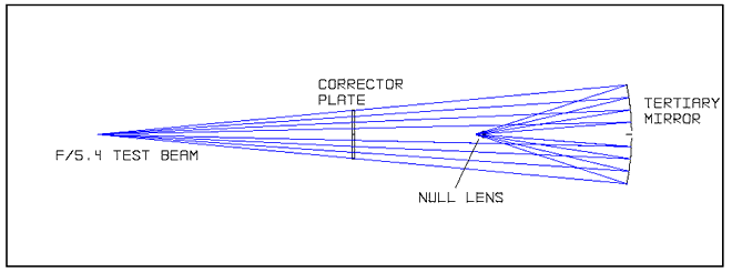
Figure 15 - Null Lens test setup

The test set-up uses a f/5.4 beam; this completely fills both the Corrector plate and the Tertiary Mirror. The source is at a distance of 2.1m from the Corrector plate, which ensures that the elements are tested at the same conjugate ratios as in the WFC. The distance from the corrector plate to the tertiary mirror is 2.278m. The test wavelength is 632.8nm.

The test beam passes through the Corrector plate and is brought to a focus by the Tertiary Mirror. Just before the focus, the beam passes through a null lens, which corrects for the aberrations introduced by the Corrector plate and Tertiary Mirror. A spherical mirror is placed so that it is concentric with the focus from the tertiary mirror. This retro-reflects the beam back through the null lens, off the tertiary mirror, through the corrector plate and back to the original focus.

The null lens will obscure the beam and produce vignetting on the Tertiary Mirror. For the layout above, the obscuration is approximately 70mm diameter on the tertiary mirror.

The diagram below shows the null lens in more detail. The null lens consists of two BK7 elements and a spherical mirror.

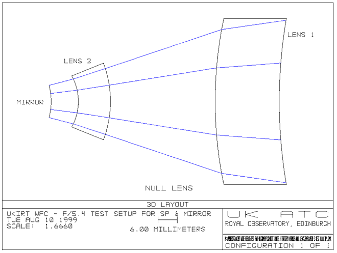
Figure 16 - Detail of null lens

The plot below shows the double pass OPD through the system. The P-V OPD is 0.0264 and the RMS OPD is 0.0076.

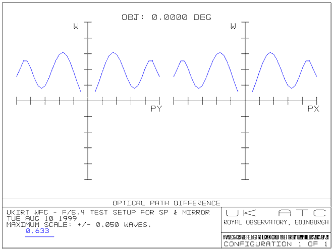
Figure 17 - Null lens performance

10.2 Focal Plane Alignment

Alignment of the four detector arrays in the focal plane unit is particularly challenging. The tolerance on co-planarity of the detector arrays is likely to be on the order of ±20mm.

It is likely that each detector array will be mounted in a cell, which is then machined so that when the cells are fitted into the focal plane unit, the arrays are co-aligned.

One possible technique is to use a combination of interferometry and microscopy. The detector active material (HgCdTe) reflects a reasonable amount of light at 0.633nm. A parallel beam interferometer could then be used to measure the flatness of the individual arrays, and the relative tilts between arrays. The tilts can then be adjusted for on each cell. This leaves the four arrays parallel to each other, but at different heights. A precision travelling microscope or optical autocollimator can then be used to measure the height differences between the arrays.

Appendix A - Optical Prescription