WFCAM SCIENCE ARCHIVE

DATA FLOW DOCUMENT

Nigel Hambly, Andy Lawrence, Ian Bond & ...

Wide Field Astronomy Unit (WFAU), Institute for Astronomy, University of Edinburgh

Modification history:

Version	Date	Comments
Draft	Oct 2002	Original version (NCH, AL & IAB)
V1.0	Jan 2003	Revised (NCH)

INTRODUCTION

The purpose of this data flow document (DFD) is to examine data transfer rates, accumulating data volumes, data formats and data curation issues for the WFCAM Science Archive (WSA) project. This, in turn, is intended to inform the hardware and software design of the WSA. Issues to be considered include import/export rates/volumes/formats; post-processing; DBMS ingest and processing (eg. indexing); and backup/update/releases. The major goal of this document is to inform decisions concerning storage hardware and investigation of network connectivity.

In this context, we consider the `flow' in data flow as encompassing i) import, ii) curation, and iii) use (including export); where `data' encompasses pixels/catalogues/housekeeping information for both WFCAM and complementary datasets (see the SRD). The DFD is organised into Sections following these three broad categories.

An overview of the end-to-end data flow, including data rates and accumulation volumes, is given in Appendix A.

IMPORT

Import data volumes and rates

Import procedure

Import formats

CURATION

Additional processing

DBMS ingest (catalogues and housekeeping data)

Additional processing in DBMS

• indexing
• sorting
• spatial index computation

Storage of pixel data

• Compression
• `Unit' of storage

Backup

Updates/releases/reruns

USE

Workspace

Access restrictions

Export formats

Export rates

End-to-end Overview

This section examines the end-to-end data flow for the UKIRT WFCAM project in order to estimate

• online storage requirements
• offline storage requirements
• network bandwidth/media requirements for data transmission
• backup media/frequency requirements

In schematic outline, the putative data flow will be along the following lines:

Assumptions

The following assumtions can be made about WFCAM; these are unlikely to change:

• the maximum data rate from the DAS is one 4-device `footprint' per 10s;
• the DAS will output 4 bytes per pixel;
• the DAS will co-add sky limited sub-exposures when a single demand exposure (specified for observing efficiency reasons for example) would saturate in the sky (eg. 40s demand integration at K);

Here, the `DAS' ($\equiv$Data Acquisition System) consists of the device itself, the device controller, and ADC and a PC system that processes the 16 bit/pixel reads from the ADC. There will be four such subsystems operating in parallel, one per WFCAM device. The PC will coadd individual 16-bit reads, or process non-destructive reads etc., and for generality will always output 32 bit values $\equiv$4 bytes/pixel (note: these PCs should not be confused with those that will operate the summit pipeline). We further assume that the individual sky-limited sub-exposures will not be kept. For the purposes of estimating both the maximum and typical data volumes/rates, the following further assumptions can be made:

• online archive will not utilise any `lossy' compression to reduce pixel storage requirements;
• UKIDSS ($\sim700$ night combined science programme) is typical of the science that will be undertaken with WFCAM;
• assume $2\times2$ microstepping and WFCAM project scientist efficiency estimates for the purposes of time-average numbers (eg. the UKIDSS proposal);
• the PEAK data rate is that delivered by the DAS maximum and using a $2\times2$ microstep mode with efficiency 0.65. An interlaced frame will be produced in $\sim1$ minute comprising 4 detectors $\times$ $2048\times2048$ pixels $\times$ 4 bytes per pixel $\times$ $2\times2$ microsteps = 270 Mbyte or 230 Gbyte per perfect 14 hour winter night;
• Typical time-averaged data rate can be estimated by averaging over UKIDSS component surveys, assuming an average 10 hour night and scaling the data rate in the previous item by the relative survey efficiencies:

  
  LAS      183.4 nights  160 Gbyte per night = 29.3 Tbyte 
  
  
  GPS      		 130.2           		  92                   		 12.0 
  
  
  GCS      		  58.8          		 160                    		 9.4 
  
  
  DXS      		 123.9           		  52                   		 6.4 
  
  
  UDS      		 130.2           		  52                    		 10.8 
  
  
  
  
  Totals: 		 $\sim700$ $\sim70.0$ 
  
  
  

  or an average over the science programme of $\sim100$ Gbyte per full night.
• data volumes/rates will include a 10% overhead on pixel data alone, where appropriate, for the purposes of allowing for derived object catalogues, housekeeping and DBMS

This last item needs closer inspection. Appendix D lists the baseline set of parameters per detected object from CASU standard pipeline processing. Assuming 4 bytes per parameter (they will be mainly single precision floating point numbers) this is 66 parameters $\times$ 4 bytes = 264 bytes per detection. Further, for the purposes of list-driven co-located photometry (see the SRD; ie. given a detection in one passband, what are the object parameters at fixed positions using fixed apertures and profiles in all other passbands) this value should be scaled appropriately for $\sim4$ UKIDSS passbands (and ultimately another 5 SDSS passbands for total generality; again, see the SRD). So, to order of magnitude, the catalogue records size is $\sim10^3$ bytes per detected object. Now, the number of detected objects per frame will vary enormously. For example, in the UKIDSS GPS, towards the Galactic centre the surface density of sources is likely to be $>10^6$ per sq. deg. (or $\sim10^{-2}$ objects per pixel) while in the lowest surface density regions of the LAS this is likely to drop to $\sim10^3$ per sq. deg. (or $\sim10^{-5}$ objects per pixel). If we assume a typical surface density of sources as being $\sim10^4$ per sq. deg., or $\sim10^{-4}$ objects per pixel, then for a given amount of pixel data the object catalogue overhead is

$$\frac{10^3 {\rm bytes/obj}\times10^{-4}{\rm obj/pix}}{4{\rm bytes/pix}}\times100\approx3\%.$$

Allowing for housekeeping, other ancilliary data and DBMS overheads, a figure of 10% overhead on pixel data does indeed seem reasonable.

Details

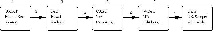
Some relevant details on individual parts of the data flow scheme above:

1,2,3: JAC/ATC responsibility; JAC will likely make offline tape archive of raw pixel data; couple of weeks online buffer storage will probably be used; ATC proposes 4-way parallelisation of the DAS & summit pipeline data chains; output format will be Starlink NDF (JAC archive) and MEFs (multi-extension FITS files) for transport to CASU.

4: For ease of housekeeping/transport/handling, one disk or tape per night would be advantageous. Peak data rate is 230 Gbyte/night. One or two disks may be employed to ship the data; alternatively tapes may be used. Currently, the highest capacity system would appear to be `Linear Tape Open' (LTO) which can store $\sim100$ Gbyte native, and would probably manage a night's worth of data (with a bit of lossless compression) on all but the most productive of nights. The transfer rate for LTO is reportedly 100 Gbyte/hour. By the time WFCAM becomes operational, there may be higher capacity in this system, or higher capacity alternatives.

5: CASU pipeline will derive/add data to the images ingested from JAC: i) housekeeping info; ii) object catalogues; iii) confidence arrays. As stated in the assumptions above, a 10% increase on pixel data volume will allow for housekeeping, object catalogues and DBMS overheads; however iii) is potentially a large increase on raw pixel volume/rates. For example, if a 2-byte confidence value per 4-byte pixel is added for any image that is likely to be stacked (cf. current CIRSI pipeline processing) then volumes/rates increase by 50%. The greater fraction of the UKIDSS science program will be stacked to increase depth, so a conservative assumption would be to increase ALL pixel data volumes/rates by a factor 1.5; however it is unlikely that confidence values will be needed on a pixel-by-pixel basis; rather nightly library confidence frames will suffice. In this case the overhead will be small and can be subsumed into the existing 10% overhead.

7: An estimate of the yearly rate can be made as follows. Nights per year are likely to be $365\times$ 80% UK time on UKIRT $\times f_{\rm WFCAM}$, the fraction of all UK time given over to WFCAM. Assume 110 Gbytes per night average, and for the likely range assume $0.6< f_{\rm WFCAM}< 0.8$. Then, the average yearly data accumulation rate will be between 19 and 26 Tbytes.

For science archiving, it is important to distinguish between storage requirements for `immediate' access (or `as fast as possible' access) and storage for less time critical usages. An examples of the former is where an astronomer wishes to trawl object catalogues for rare objects, where data exploration (ie. interaction in real time) is important. An example of the later is where a `power user' wishes to reprocess a large fraction of survey data to look for objects that they believe were missed in the standard pixel processing pipeline (eg. large-scale, low surface brightness objects). The split in usages requiring fast/slower (real-time/offline) response times is a split between catalogue usage and pixel data usages, broadly speaking.

An estimate of the final pixel storage requirement for UKIDSS at least is straightforward: assuming 4 bytes per pixel and $2\times2$ microstepping (ie. 0.2 arcsec pixels); the areas of the LAS, GPS, GCS, are respectively 4000 sq. deg. $\times5$ filters; $1800\times5$; $1600\times4$ (stacked pixel data for the DXS and UDS are negligible for these purposes). This adds up to $\sim50$ Tbytes; the final UKIDSS object catalogues and associated data will be $\sim5$ Tbytes.

At each point in the end-to-end system, the data flow volumes/rates and some hardware requirements can be roughly stated as follows:

1,2,3:

• Peak data rate 230 Gbyte/night
• Average data rate 100 Gbyte/night for $\sim200$ nights each year
• Accumulation of data: $\sim20$ Tbyte/year
• Online storage requirements (summit): a few Tbytes

Nightly backups required; these should be able to cope with 230 Gb/night; one backup tape per night if possible; $\sim200\times{\rm N}$ tapes needed per year for JAC offline raw data archive, where N = no. of tapes per night.

4:

• Peak data rate: 230 Gbyte/night
• Average data rate 100 Gbyte/night for $\sim200$ nights each year
• One disk or tape per night if possible

If a tape solution were to be employed, and furthermore those tapes were used as an offline backup at CASU (as opposed to being recycled) then $\sim200\times{\rm N}$ tapes would be needed per year for data transfer to CASU and subsequent shelving in CASU UKIRT data archive, where N = average no. of tapes per night.

5:

• Peak data ingest rate: 230 Gbyte/night
• Average data ingest: 100 Gbyte/night for $\sim200$ nights per year

from here on, data volumes/rates multiplied by $1.1$ to account for housekeeping/catalogue overheads:

• Typical rate of accumulation of processed data: 22 Tb/year

6: If network, then need to be able to transfer 250/110 Gbyte/day (peak/average). Note: a 1 Gbit/s continuous link would enable 450 Gbyte/hr to be transfered.

7:

• Data ingest: 250/110 Gbyte/day (peak/average)
• Accumulation of data: 22 Tb/yr

Archive backup frequency: every few months probably sufficient; speed not critical but clearly 1 Tb/day may eventually become impractical as archive size increases beyond 100 Tb while 10 Tb/day may be overkill.

8: User access: SSS is Gbyte/week; suggest it is likely that WFCAM archive is likely to be 10x more, hence   Gbytes/day.

Summary for the WSA

In summary, data flow for the WSA will be:

• Ingest: $\sim250/110$ Gbyte per day (peak/average) for $\sim200$ days per year;
• Accumulation of data: $\sim20$ Tbytes per year;
• Accumulation of catalogue, housekeeping and other ancilliary data: $\sim2$ Tbytes per year.

The uncertainties above (eg. detected objects per pixel; the amount of confidence array information needed to be stored, etc.) should not prevent progress on hardware design and acquisition, since storage for the final data volume does not have to be purchased up front. Provided sufficient storage is acquired for the first year of operation, it will become clearer during that time what the precise long term requirements are. In any case, the lifetime of the WSA project is significantly longer than the typical timescale of leaps in computer hardware design, so it should be expected that the initial hardware solution will not be the final one, and a phased approach (as is required from the science exploitation point of view; see the SRD) is implied.

Descopes

Numbers above are of course dominated by the volume of pixel data. If it is decided that it is unnecessary to archive processed pixels in uncompressed form, then storage volumes & data rates can be reduced dramatically. For example, if the archive contains 10x H-compressed pixels, then all numbers from 6 onwards can be reduced by $\sim90$%. However, there is a very clear requirement in the SRD for online archiving of unadulterated pixel data.

In specifying the requirements, a chance could be taken on assumption of the average number of usable nights: eg. UKIDSS proposal suggests that on average, 70% of allocated nights will produce science data, so volumes/rates can be decreased by 30% (but note that on a daily basis the data flow system should still be able to cope with peak data rates produced by hopefully many perfect nights).

FITS headers

WFAU network connectivity

Catalogue parameter list (standard CASU processing)

APM/SuperCOSMOS/INT WFC/CIRSI analysis produces 32 4-byte parameters per detected object. This has been enhanced to include extra parameters for flux estimation and error estimates. The following is the suggested list for the standard WFCAM pipeline:

No. 		 Name 		 Description 




1 		 Seq. no. 		 Running number for ease of reference, in strict order of image detections


2 		 Isophotal flux 		 Standard definition of summed flux within detection isophote, apart from 


detection filter is used to define pixel connectivity and hence which


pixels to include. This helps to reduce edge effects for all isophotally


derived parameters.


3 		 X coord 		 Intensity-weighted isophotal centre-of-gravity in X


4 		 Error in X 		 estimate of centroid error 


5 		 Y coord 		Intensity-weighted isophotal centre-of-gravity in Y


6 		 Error in Y 		 estimate of centroid error 


7 		 Gaussian sigma 		These are derived from the three general intensity-weighted second moments. 


8 		 Ellipticity 		The equivalence between them and a generalised elliptical Gaussian distribution


9 		 Position angle 		 is used to derive Gaussian sigma = $(\sigma_a^2+\sigma_b^2)^{1/2}$ 


Ellipticity = $1.0-\sigma_a/\sigma_b$ 


Position angle = angle of ellipse major axis wrt x axis




10 		 Areal profile 1 		Number of pixels above a series of threshold levels relative to local sky.


11 		 Areal profile 2 		Levels are set at T, 2T, 4T, 8T ...128T where T is the threshold. These


12 		 Areal profile 3 		can be thought of as a sort of poor man's radial profile. Note that for now 


13 		 Areal profile 4 		deblended, ie. overlapping images, only the first areal profile is computed


14 		 Areal profile 5 		and the rest are set to -1 flagging the difficulty of computing accurate


15 		 Areal profile 6 		profiles.


16 		 Areal profile 7 		 


17 		 Areal profile 8 		 




18 		 Peak height 		in counts relative to local value of sky - also zeroth order core flux 


19 		 Error in pkht 		 




20 		 Core flux 		Best used if a single number is required to represent the flux for ALL


objects. Basically aperture integration with radius rcore (in the FITS


header) but modified to simultaneously fit `cores' in case of overlapping


images.  Best scaled to $\approx<$FWHM$>$ for site+instrument. 


Combined with later-derived aperture corrections for general photometry. 


21 		 Error in flux 		 


22 		 Core 1 flux 		A series of different radii core/aperture measures similar to parameter 20


23 		 Error in flux 		 


24 		 Core 2 flux 		Together with parameter 18 these give a simple curve-of-growth analysis from


25 		 Error in flux 		 


26 		 Core 3 flux 		peak pixel, $1/2\times$ rcore, rcore, $\surd2\times$ rcore, $2\times$ rcore, $2\surd2\times$ rcore,


27 		 Error in flux 		 $4\times$ rcore, $4\surd2\times$ rcore, $8\times$ rcore, $8\surd2\times$ rcore, $16\times$ rcore, 


28 		 Core 4 flux 		  $16\surd2\times$ rcore, $32\times$ rcore  


29 		 Error in flux 		 


30 		 Core 5 flux 		 $4\times$ basic core, ensures $\sim99$% of PSF flux


31 		 Error in flux 		 


32 		 Core 6 flux 		 Extras for generalised galaxy photometry further spaced


33 		 Error in flux 		 


34 		 Core 7 flux 		 by $\surd2$ in radius to ensure correct sampling out to 


35 		 Error in flux 		 


36 		 Core 8 flux 		 reasonable range of aperture sizes 


37 		 Error in flux 		 


38 		 Core 9 flux 		 Note these are all corrected for pixels from overlapping neighbouring images 


39 		 Error in flux 		 


40 		 Core 10 flux 		  


41 		 Error in flux 		 


42 		 Core 12 flux 		 Biggest would be $32\times$ rcore ie. $\approx$30 arcsec diameter


43 		 Error in flux 		 




44 		 Petrosian radius 		 $r_p$ as defined in Yasuda et al. 2001 AJ 112 1104 


45 		 Kron radius 		 $r_k$ as defined in Bertin and Arnouts A&A Supp 117 393


46 		 FWHM radius 		 $r_{fhwm}$ average image radius at half PeakHeight 


47 		 Petrosian flux 		 Flux within circular aperture to $k \times r_p$


48 		 Error in flux 		 


49 		 Kron flux 		 Flux within circular aperture to $k \times r_k$ 


50 		 Error in flux 		 


51 		 FWHM flux 		 Flux within circular aperture to $k \times r_{fwhm}$ - simple alternative


52 		 Error in flux 		 




53 		 Error bit flag 		 Bit pattern listing various processing error flags




54 		 Sky level 		 Local interpolated sky level from background tracker


55 		 Sky variance 		 Local estimate of variation in sky level around image


56 		 Child/parent 		 Flag for parent or part of deblended deconstruct





The following are accreted directly after standard catalog generation




57 		 RA 		RA and Dec explicitly put in columns for overlay programs that cannot, in


58 		 Dec 		general, understand astrometric solution coefficients. Derived exactly from


WCS in header and XY in parameters 5 & 6




59 		 Classification 		Flag indicating probable classification: eg. -1 stellar, +1 non-stellar, 0 noise


60 		 Statistic 		An equivalent N(0,1)  measure of how stellar-like an image is, used in


deriving parameter 59 in a `necessary but not sufficient' sense



From the further processing pipeline after deriving a suitable PSF




61 		 PSF flux 		 Fitted flux from PSF 


62 		 Error in flux 		 


63 		 X coord 		 Updated PSF-fitted X centroid 


64 		 Error in coord 		 


65 		 Y coord 		 Updated PSF-fitted Y centroid 


66 		 Error in coord 		

About this document ...

This document was generated using the LaTeX2HTML translator Version 2K.1beta (1.47)

Copyright © 1993, 1994, 1995, 1996, Nikos Drakos, Computer Based Learning Unit, University of Leeds.
Copyright © 1997, 1998, 1999, Ross Moore, Mathematics Department, Macquarie University, Sydney.

The command line arguments were:
latex2html -split 0 wsadfd

The translation was initiated by Nigel Hambly on 2003-01-08